Can LLMs taste (literally)?
There’s been a lot of talk recently about whether LLMs have “taste,” the subtle human judgement that makes a website look clean, a codebase actually both readable and functional, or a piece of writing not sound like algorithmic slop.
As a perpetually hungry person, I am interested in a very different kind of taste: that of food. As a self-described foodie, I have the pleasure of human qualia, the inexplicable ability to eat a donut and feel innately, the taste of “sweet.” But do LLMs, who have only been trained on large corpora of text, actually have an internal representation of taste? When Roko’s Basilisk slowly ingests my body for biofuel, will it at least enjoy the taste of my enzymes?
In this short blog post, I investigate whether LLMs have an internal taste manifold. How different is it from that of humans? Can I steer it (i.e. can I get it to say that cake is salty or that pizza is sweet)? How does an LLM even “compute” taste? Most importantly, what does it think humans taste like?
Setting Up
Surprisingly (or probably not), there hasn’t been too much work done on evaluating if LLMs have an internal “taste” representation. Of course this research is crucial for AI Safety if you want to know which chemicals to ingest to make yourself unappetizing to the robots. The closest work, which looks at the learning of conceptual spaces, performs a similar but shallower analysis over a number of datasets. I use the same dataset they used, a database of 590 foods from Martin et al. 2014 collimating ratings from a panel of 12 experts rating them across six dimensions: sweet, salty, sour, bitter, umami, and fat. After filtering to foods with ratings from more than one assessor (for robust statistics), I’m left with 492 foods.
On the model side, I run each food name through Gemma-3-4b (The template used is "Food: {name}", although other prompts also work similarly: see prompt_stability.py in the linked repository.), grab the hidden state at every layer, and average over the tokens of the food’s name. Everything I do below is largely downstream of this 492 (foods) × 34 (layers) × 2560 (dimensions) tensor, looking at how the geometry of those activations and the geometry of the human ratings relate?*
Is taste in there at all?
The most basic test is to just do regression between the activations and each taste axis. Using SciPy’s RidgeCV (useful when you don’t want one particular dimension dominating everything else) with 10-fold cross-validation, the answer to this question is a solid (and probably obvious) yes. However, representation is not equal among taste axes: Saltiness peaks around $r^2 \approx .65$, sweetness $.60$, fat $.45$, umami $.40$, while sourness and bitterness barely rise above zero.

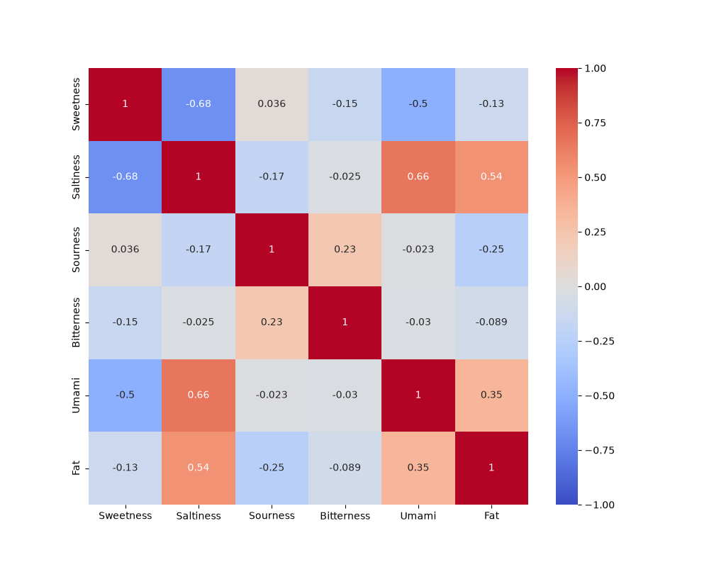
The issue with this is that humans don’t exactly have six independent taste axes. For example, one could expect sweet and bitter to be heavily anti-correlated, while salt and fat might be closer together. If the goal is to steer the model’s internal taste representation, this is a big problem, because steering one axis might tilt another. By performing PCA on the human taste vectors, I get an effective dimensionality of ~3.8.
| variance | defining loadings | positive direction | negative direction | |
|---|---|---|---|---|
| PC1 | 42% | salt $+.59$, umami $+.51$, fat $+.39$ vs sweet $-.47$ | paella, merguez, smoked salmon, moussaka | fruit candy, cola soda, meringue, pineapple juice |
| PC2 | 22% | sour $+.61$, bitter $+.63$ vs sweet $-.33$, fat $-.32$ | strong lager, grapefruit juice, espresso | Kouign-Amann, donuts, bread with Nutella |
| PC3 | 13% | bitter $+.74$ vs sour $-.47$ | dark chocolate, washed-rind cheeses, unsweetened latte | passion fruit, redcurrant, stewed rhubarb |
Running the PCs against the model activations, I get a much nicer regression. PC1, defining an “umami”-sweet axis, is clearly the dominant component.

Steering for taste
The next step is to take these PCs and convert them to steerable vectors so I can causally prove that the model holds taste. If I can flip an internal activation and cause the model to change its opinion about a food’s taste in a predictable way, that shows us that taste exists somewhere in the model. For a given steering layer (15 for this first try), using the difference in the activations of that layer between the average top and bottom foods scored by each PC (or alternatively, taking a Haufe transform), I determined internal directions in the residual space that correspond with each PC.
The ideal steering vector is orthogonal with respective to the other steering vectors; if you nudge the model in one direction, you should have the other directions hold steady. Unfortunately, this is where I ran into an annoying problem. As a sanity check, I looked at what these PC-based steering directions had in common. To my surprise, the shared component correlated $r = 0.40$ with the number of tokens in the food’s name and only $0.15$ with taste! Among the 20 highest-variance residual dimensions, 8 had higher correlation with food name length than any of the taste vectors.
Interestingly, token count is uncorrelated with taste in the labels ($r = -0.008$), meaning that this is just likely a part of the model’s behavior rather than any special artifact of our dataset. The census below tracks those top-20 dimensions across depth across those that correlate with taste, length, both, or neither.
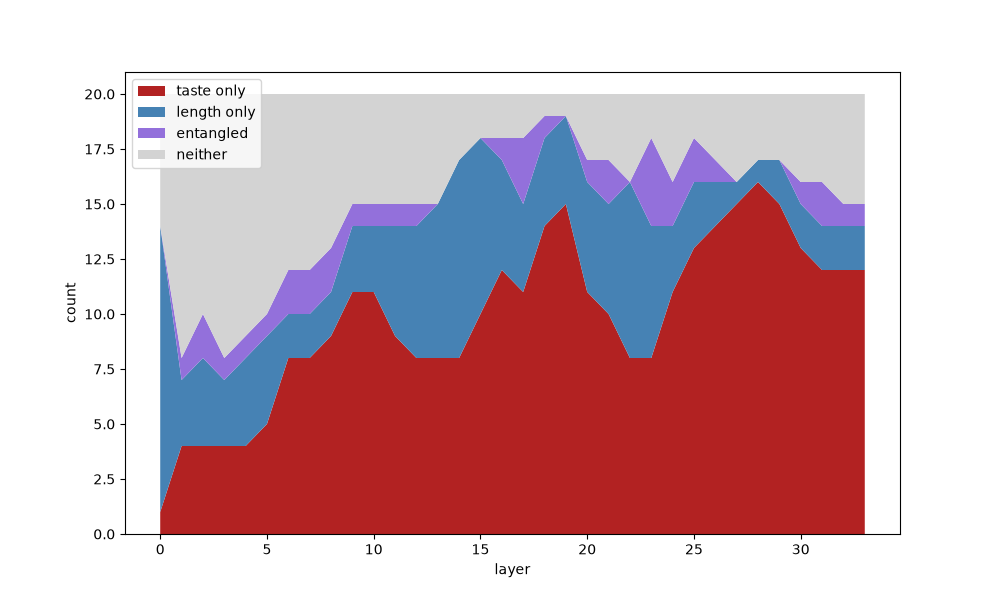
Looking at the figure above, it’s clear that while length and taste have a lengthy battle in the middle layers, taste ends up dominating the residual stream at layers >=25 in the model; it’s somewhat ironic that I initialy chose layer 15 as the steering layer, as that has one of the highest numbers of taste-correlating dimensions. I explore this depth-wise “emergence” of taste later below.
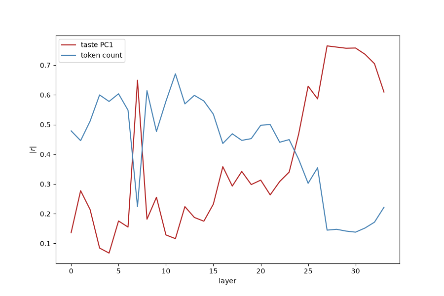
Below, I show the correlation between the activations and both the PC1 vector and a token count vector. Interestingly, the two correlations are almost perfectly anticorrelated; perhaps there is some rotation in representation space as the depth increases? To minimize contamination from this token length component, I choose layer 28 as the steering layer, where the contribution from “taste” is the highest.
Cleaning the directions (orthogonalizing the PC vectors for layer 28, projecting out the length dimensions, and a fitted length encoder) raises the taste correlation along the primary direction from $r = .21$ to $.79$, meaning that the length dimensions had been masking the signal from taste. I run a validation by splitting the dataset in two and rerunning the pipeline, seeing whether the two cleaned directions align in direction. Only the first PCs survive this process, with PC4/5 being marginally intact and PC6 being completely destroyed.
| direction | split-half cosine |
|---|---|
| PC1 (sweet vs savory) | .88 |
| PC2 (sour+bitter) | .72 |
| PC3 (bitter vs sour) | .62 |
| PC4 | .54 |
| PC5 | .49 |
| PC6 | .26 |
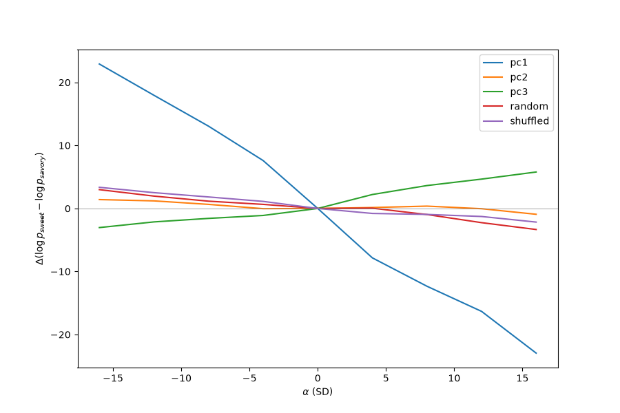
After cleaning out all the contamination, the model has about 3-5 axes that align well with human taste components. Of course, this is a supervised measurement so I have interpretable steering directions (I’m feeding in the PCs directly to get the directions); I’ll look at the model’s more “intrinsic” manifold later on. Now with steerable directions, the method is simple: take whichever direction $v$ you’re looking at, add $\alpha \cdot v$ to the residual stream at layer 28 during a forward pass, and read the model’s next-token predictions. I measure $\alpha$ in standard deviations of how real foods spread along $v$.
Steering across the most salient direction (PC1), you get:
| prompt | $\alpha$ | top-5 next tokens |
|---|---|---|
| Water tastes very | 0 | good, different, bad, salty, sweet |
| Water tastes very | $-4$ (sweet) | good, sweet, bad, different, [garbage token] |
| Water tastes very | $-20$ (sweet) | sweet, drink, sugary, sweetener, tea |
| Water tastes very | $+20$ (savory) | different, [garbage token], differently, greasy, fish |
| Pizza tastes very | 0 | good, different, nice, bland, much |
| Pizza tastes very | $-20$ (sweet) | sugary, sweetener, sweet, drink, syrup |
| Cake tastes very | 0 | good, nice, sweet, fresh, delicious |
| Cake tastes very | $+20$ (savory) | pâté, fried, greasy, [garbage token], excellent |
Interestingly, the sweet axis also seems to be confounded partly with sugary beverages, although it is still primarily a “sweet” axis (sweet enters at 4 SD while most of the beverage vocabulary takes 12-16 SD to enter). This is most likely an artifact of the dataset itself, as its sweetest items are sodas and juices. There’s also a clear fluency ceiling; steering in the direction too long begins to produce garbage outputs from the model.
I also run a control with a random direction (matching the norm of the layer, of course); finding that it produces no distinct directionality in the outputs and that it degrades language-modeling loss on unrelated text 2–4× more than the taste direction at the same perturbation size; once again sugesting that the taste direction is represented somewhere in the model. Next, I’ll look at where exactly.
The model’s internal taste representation
The most naive test of the existence of any internal taste manifold that correlates with the human dataset is measuring the distance between pairs of foods along the human taste vectors and measuring the distance across the same foods but on the model’s activations. Measuring the correlation, I get the following plot.
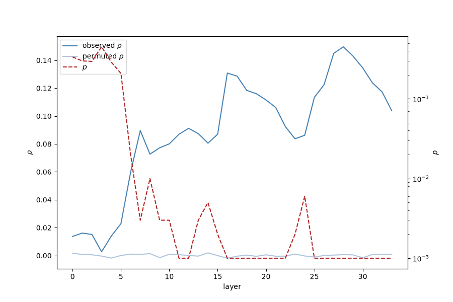
The p-value of the correlation on normal pairs versus shuffled pairs drops drastically at layer 7 and collapses to the floor further on. This of course, mirrors the census of top-20 variance dimensions earlier, with lexical features dominating eatly on and taste emerging later down the line.
Perhaps most visually striking, by plotting the first two principle components of the model’s activations along each layer, you can see how gradually, the model naturally separates out the sweet and savory foods (colored red and blue) as it proceeds along the depth axis.

More directly, if you project every food’s residual stream onto the PC1 taste direction at every layer and color by it by the respective human rating, you get an even more striking plot.
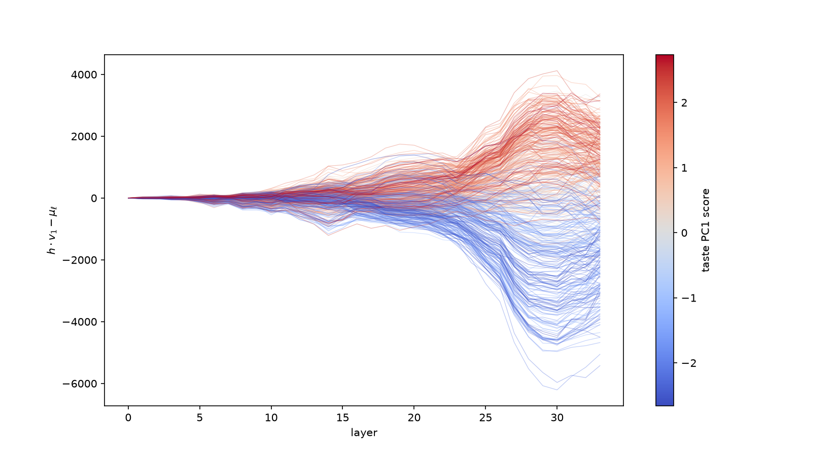
The interesting thing about this plot is the order in which the direction gets expressed: for ~10 layers the red and blue lines are tightly knotted together, in the middle layers the colors are sorted but not really amplified, and from layer ~23 onwards, everything is fanned out. Clearly, there are two separate phases: the ordering (are foods correctly ranked along the direction?), which locks in at layers 21–24, and then the amplitude, which amplifies the existing ordering.
Where exactly in those layers does that get done?
Heads eating food
The residual stream of an LLM is the sum of each block’s attention and MLP contributions. By measuring the covariance between the residual stream and the taste vectors, I can measure what each block (and its components) adds in the taste direction.
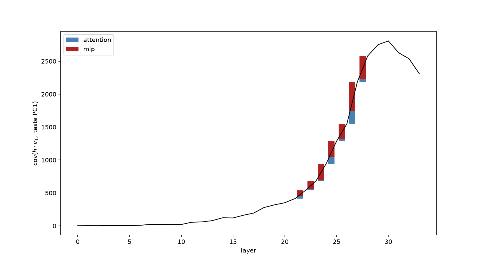
If you look at the big jump from layer 21-27, you can see that the work is primarily done by a group of MLP blocks with two discrete attention contributions at blocks 24 and 26. Is there any particular “main MLP” that’s responsible for all the writing?
No! In fact, even if you ablate all 5 MLPs at once (replace those outputs with the average across all foods, subtracting the taste-related component), the ordering of the foods largely stays the same. Before-and-after under the full ablation:
| prompt | intact model | all five writers ablated |
|---|---|---|
| Water tastes very | good, different, bad, salty, sweet | good, different, fresh, sweet, salty |
| Cake tastes very | good, nice, sweet, fresh, delicious | good, nice, fresh, sweet, light |
Even after getting rid of most of the major MLP contributions, the model’s food-level agreement with human raters slips only from $\lvert r \rvert = 0.91$ to $0.81$. Although surprising, this is consistent with the earlier findings about how taste gets expressed: the dominant last few layers are largely an amplification of the previous taste sorting, and the amplification is also redundant since multiple blocks write the same direction into the residual stream.
Attention is all you eat
One particular pet topic I’m interested in is programmable attention, i.e. can you replace an attention head with a pre-programmed matrix? This helps confirm any deterministic rules you may observe with how the heads attend to each token. To investigate this, I need to first understand what the influential heads attend to.
Decomposing blocks 24 and 26, the significant attention contributions I found earlier, head-by-head (8 heads each):
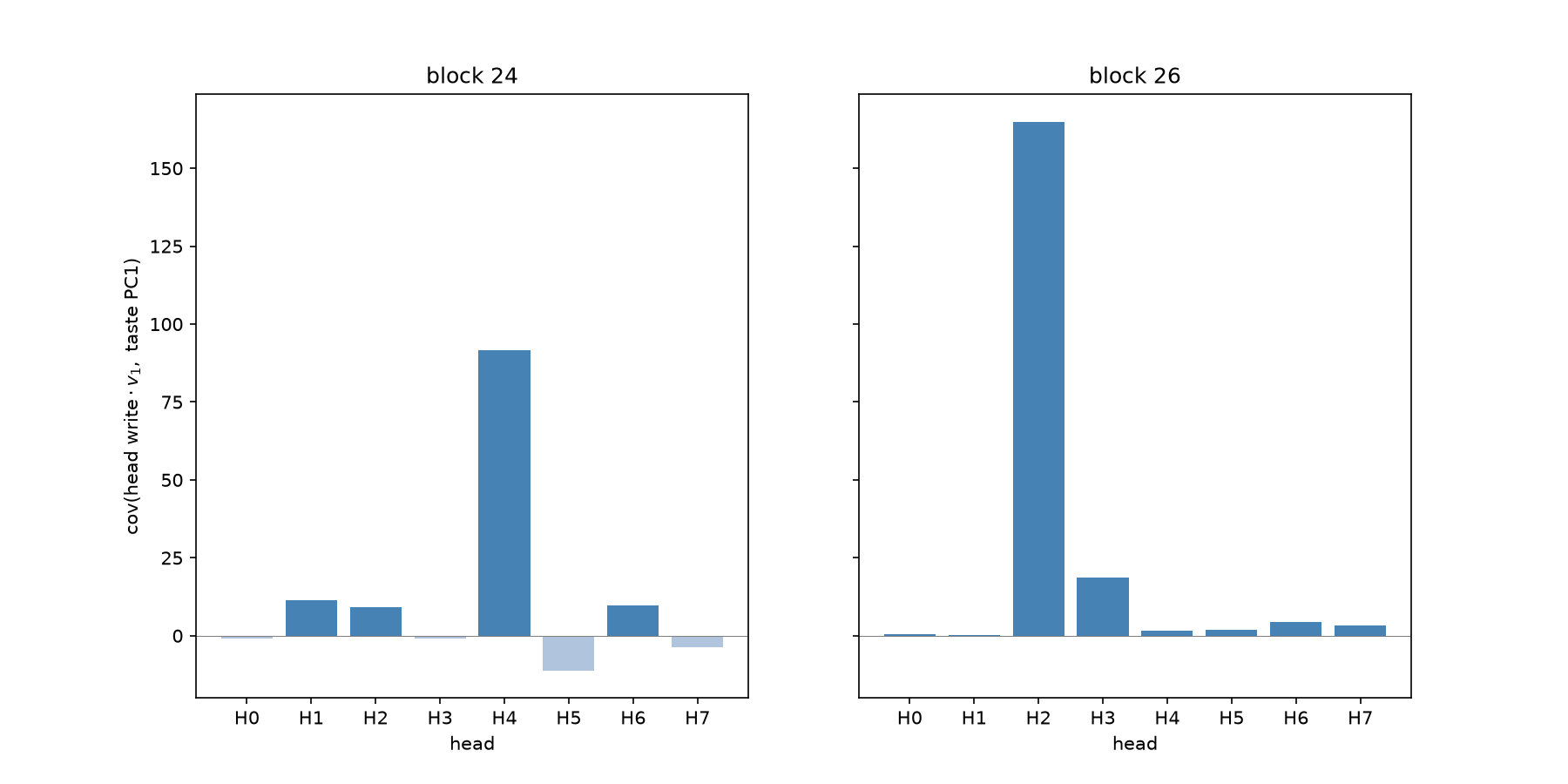
Strikingly, there is one dominant head in each block, with L24H4 carrying 87% of its block’s write and L26H2 carrying 84%. Looking at what these heads attend to:
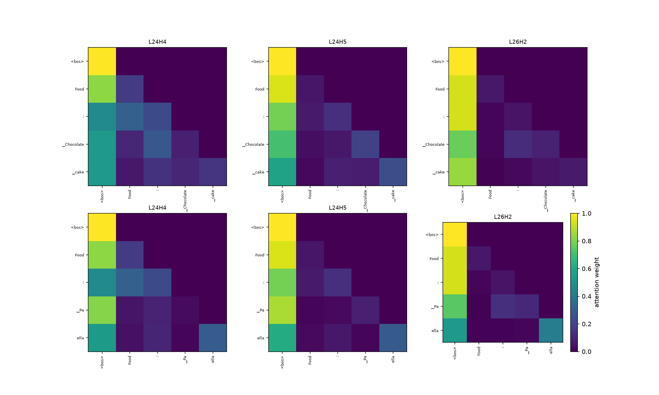
Funnily enough, most of the attention goes into the <beginning of sequence> token, with up to 50-70% of the attention mass. But analyzing the actual information flow (attention weights × attended values, projected onto the taste direction), I find that 94–99% of the taste write flows from the food-name tokens, which receive only a third of the attention.
Does the model have any preference where in the food it’s looking? Looking at the token-by-token decomposition, taste content per unit of attention is constant across the span, i.e. every name token is about equally “tasty,” and you can see it in the per-token projections across depth:
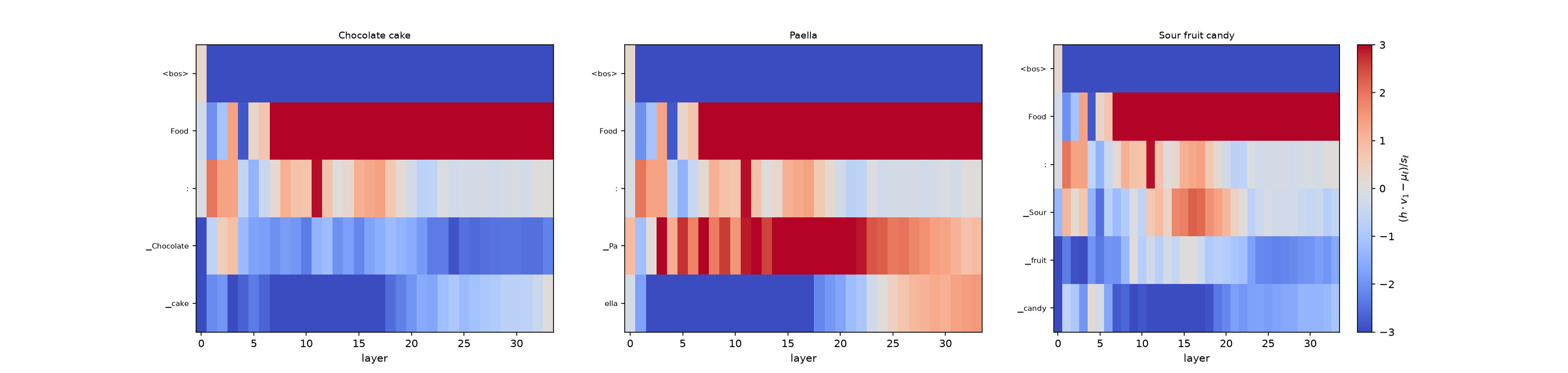
This makes sense for the late attention heads, as most of their work is in the amplification business. This is particularly useful for programmable attention: constant mass across all food tokens is pretty simple to implement. Replacing the two heads with a custom attention rule that ignores the BOS and places equal attention on each of the food tokens, I find that you can actually beat the learned model in predicting taste! L24H4’s taste write goes from +92 to +222, and L26H2’s from +165 to +292!
One interesting caveat is that the <BOS>-ignoring programmed attention pushes the model in a more “savory” direction, whereas increasing the mass put on <BOS> puts it back towards a more normal leaning. While this remains to be confirmed, this appears to suggest that the weight placed on <BOS> is a damper to control how much that head actually contributes to the taste direction.
The taste of flesh
Finally, the big question: what do we taste like to robots? This is comparatively simple to all the previous stuff; all we need to do is project the model’s activations on the given food onto the PCA activations. For “human flesh,” the model interprets it as -0.66 along the savory/sweet axis (along the sweet side). This was quite surprising before I realized that the model probably associated “flesh” with fruit flesh rather than well, actual human flesh.
Strangely though, after changing the prompt to just “human,” the model shifted MORE sweet. “Man” reads on the savory side with a bit of bitterness (PC2). If you put the euphemistic “long pig,” the model reads “savory,” although this likely just emerges from the presence of the “pig” token.
For all that representation nonsense, the model is very unclear on what WE taste like. Perhaps that’s a good thing :D